Finding STk vs. Tk sequence determinants

In this example, we’ll tackle a problem of multiple sequence alignment (MSA) sequences’ classification.

Protein kinases (PKs), or phosphate transferases, are regulatory enzymes ubiquitous across all major known taxae. They catalyze transferring of phosphate moieties from an ATP molecule to the carboxylic group of an amino acid residue. This changes physicochemical properties of a target protein, altering it’s overall behavior and functionality. Thus, they act as molecular controllers, deeply embedded into regulating mechanisms governing complex cellular machinery.

Over the course of evolution, along with substrate specificity, PKs developed a preference towards certain amino acid residues (Fig. 1). The principal group of PKs that likely appeared initially were PKs transferring phosphate to serine and threonine residues (STk). Later, another group emerged, specializing towards the tyrosine residue (Tk).

Fig. 1. Phosphorylation of Ser/Thr and Tyr. Notice the dissimilarities between these two groups

What could be the sequence differences enabling such a specialization? Could we find them using features selection machinery?

In 1994, Juswinder performed a conservation-based analysis of STk and Tk sequences (use this link for a full paper). He discovered several MSA positions that, as structural evidence suggests, exploit physicochemical differences (e.g., volume) between Ser/Thr and Tyr. For this, he used a scoring function that would spot positions with substantial but different conservation between STk and Tk sequences in the same multiple sequence alignment.

---

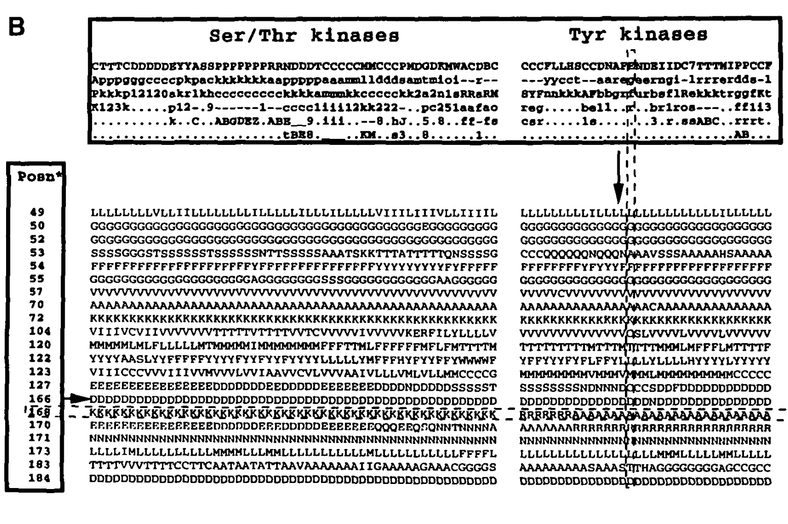
Fig. 2. Positions of STk ad Tk sub-alignment (note 201 and 203)

---

Fig. 2. Positions of STk and TK sub-alignment part2 (note 168 and 170)

---

Here, we’ll attempt to recover positions highlighted by Juswinder on a larger MSA built from reviewed UniProt sequences.

# ! pip install lXtractor eBoruta ipywidgets xgboost

import gzip
import re
from collections import Counter
from io import StringIO, BytesIO
from itertools import chain

import lXtractor.chain as lxc
import lXtractor.variables as lxv
import pandas as pd
from lXtractor.ext import PyHMMer
from lXtractor.util import fetch_text
from more_itertools import consume

The UniProt link is generated from the search API. We are taking all reviewed proteins (Swiss-Prot database) belonging to the PK superfamily.

Link to Pfam points to the PF00069 – a protein kinase domain HMM profile.

LINK_UNIPROT = "https://rest.uniprot.org/uniprotkb/stream?fields=accession%2Cid%2Csequence%2Cft_domain%2Cprotein_families&format=tsv&query=%28%28family%3A%22protein%20kinase%20superfamily%22%29%29%20AND%20%28reviewed%3Atrue%29"
LINK_PFAM = 'https://www.ebi.ac.uk/interpro/wwwapi//entry/pfam/PF00069?annotation=hmm'

text = fetch_text(LINK_UNIPROT)

df_up = pd.read_csv(StringIO(text.decode('utf-8')), sep='\t')

df_up.head()

	Entry	Entry Name	Sequence	Domain [FT]	Protein families
0	A0A075F7E9	LERK1_ORYSI	MVALLLFPMLLQLLSPTCAQTQKNITLGSTLAPQGPASSWLSPSGD...	DOMAIN 22..149; /note="Bulb-type lectin"; /evi...	Protein kinase superfamily, Ser/Thr protein ki...
1	A0A078CGE6	M3KE1_BRANA	MARQMTSSQFHKSKTLDNKYMLGDEIGKGAYGRVYIGLDLENGDFV...	DOMAIN 20..274; /note="Protein kinase"; /evide...	Protein kinase superfamily, Ser/Thr protein ki...
2	A0A0B4J2F2	SIK1B_HUMAN	MVIMSEFSADPAGQGQGQQKPLRVGFYDIERTLGKGNFAVVKLARH...	DOMAIN 27..278; /note="Protein kinase"; /evide...	Protein kinase superfamily, CAMK Ser/Thr prote...
3	A0A0K3AV08	MLK1_CAEEL	MEQASVPSYVNIPPIAKTRSTSHLAPTPEHHRSVSYEDTTTASTST...	DOMAIN 69..130; /note="SH3"; /evidence="ECO:00...	Protein kinase superfamily, STE Ser/Thr protei...
4	A0A0P0VIP0	LRSK7_ORYSJ	MPPRCRRLPLLFILLLAVRPLSAAAASSIAAAPASSYRRISWASNL...	DOMAIN 389..661; /note="Protein kinase"; /evid...	Leguminous lectin family; Protein kinase super...

Initialize profile as PyHMMer object internally interfacing homonimous library. PyHMMer is an annotator class, annotating (subsetting) ChainSequences using HMM-derived domain boundaries.

prof = PyHMMer(BytesIO(gzip.decompress(
    fetch_text(LINK_PFAM, decode=False)
)))

Initialize ChainSequences and wrap them into the ChainList. The latter simplifies working with a group of Chain*-type objects. To learn more, check lXtractor documentation.

def wrap_into_chain_seq(row):
    """
    :param row: DataFrame row.
    :return: chain sequence using "Sequence" field to obtain a full
        protein sequence and "Entry Name" for its name.
    """
    fam_df = row['Protein families']
    family = 'other'
    if 'protein kinase family' in fam_df:
        if 'Ser/Thr' in fam_df:
            family = 'STk'
        elif 'Tyr' in fam_df:
            family = 'Tk'

    return lxc.ChainSequence.from_string(
        row['Sequence'], name=row['Entry Name'], meta={'Family': family}
    )

chains = lxc.ChainList(
    wrap_into_chain_seq(r) for _, r in df_up.iterrows()
)
Counter(c.meta['Family'] for c in chains)

Counter({'STk': 3702, 'Tk': 551, 'other': 248})

Select only those whose family was classified as STk or Tk.

chains = chains.filter(lambda x: x.meta['Family'] != 'other')

Below, alignment-extracted boundaries are used to create a “child” subsequence for each ChainSequence in chains. We also specify acceptance criteria: minimum length of extracted domain, minimum coverage, i.e., how many HMM positions were covered by the extracted sequence, and minimum bit score (which is a bit higher than the profile’s own threshold; just to be safe).

consume(prof.annotate(
    chains, new_map_name='PK', min_size=150, min_cov_hmm=0.7, min_score=50
));

len(chains), len(chains.collapse_children())

(4253, 3911)

We observe that the final number of chains with annotated domains under the filtering criteria specified above differs from the initial number of chains. UniProt obtains PK domain annotations using a different profile using ProSite software. Thus, the filtering criteria are essentially sensitivity tweaks.

chains = chains.filter(lambda x: len(x.children) > 0)
len(chains), Counter(c.meta['Family'] for c in chains)

(3861, Counter({'STk': 3406, 'Tk': 455}))

We encode the alignment using the ProtFP embeddings derived from the PCA of the AAIndex database. Thus, they encapsulate many physicochemical properties in several compact dimensions.

# The number of PCA components to take.
N_COMP = 3

Define variables – N_COMP PCA components for each profile position. lXtractor is shipped with values already and the “calculation” of variables below is simply accessing the table values for each valid residue. By default, NaN used as a placeholder for empty values (gaps in the sequence-to-profile alignment).

variables = list(chain.from_iterable(
    (lxv.PFP(pos, i) for i in range(1, N_COMP + 1)) for pos in range(1, prof.hmm.M + 1)
))
len(variables)

789

manager = lxv.Manager(verbose=True)
calculator = lxv.GenericCalculator()  # You may increase the number of processes here.
domains = chains.collapse_children()
df = manager.aggregate_from_it(
    # `calculate` returns a generator of the calculation results.
    # We immediately aggregate the results into a single table.
    manager.calculate(domains, variables, calculator, map_name='PK'),
    num_vs=len(variables)
)

Finally, incorporate labels for STk (0) and Tk (1) domain sequences.

cls_map = {'STk': 0, 'Tk': 1}
id2cls = {s.id: cls_map[s.parent.meta['Family']] for s in domains}
df['IsTk'] = df['ObjectID'].map(id2cls)

df.head()

	ObjectID	PFP(p=1,i=1)	PFP(p=1,i=2)	PFP(p=1,i=3)	PFP(p=2,i=1)	PFP(p=2,i=2)	PFP(p=2,i=3)	PFP(p=3,i=1)	PFP(p=3,i=2)	PFP(p=3,i=3)	...	PFP(p=261,i=1)	PFP(p=261,i=2)	PFP(p=261,i=3)	PFP(p=262,i=1)	PFP(p=262,i=2)	PFP(p=262,i=3)	PFP(p=263,i=1)	PFP(p=263,i=2)	PFP(p=263,i=3)	IsTk
0	PK_1|526-791<-(LERK1_ORYSI|1-813)	NaN	NaN	NaN	NaN	NaN	NaN	NaN	NaN	NaN	...	NaN	NaN	NaN	NaN	NaN	NaN	NaN	NaN	NaN	0
1	PK_1|20-274<-(M3KE1_BRANA|1-1299)	3.14	3.59	2.45	5.11	0.19	-1.02	5.76	-1.33	-1.71	...	-3.82	-2.31	3.45	7.33	4.55	2.77	6.58	-1.73	-2.49	0
2	PK_1|27-278<-(SIK1B_HUMAN|1-783)	3.14	3.59	2.45	-6.61	0.94	-3.04	6.58	-1.73	-2.49	...	-2.79	6.60	1.21	7.33	4.55	2.77	5.11	0.19	-1.02	0
3	PK_1|205-445<-(MLK1_CAEEL|1-1059)	NaN	NaN	NaN	NaN	NaN	NaN	NaN	NaN	NaN	...	NaN	NaN	NaN	NaN	NaN	NaN	NaN	NaN	NaN	0
4	PK_1|392-592<-(LRSK7_ORYSJ|1-695)	NaN	NaN	NaN	NaN	NaN	NaN	NaN	NaN	NaN	...	NaN	NaN	NaN	NaN	NaN	NaN	NaN	NaN	NaN	0

5 rows × 791 columns

For convenience, we’ll define several helper functions and a Dataset dataclass holding the full dataset.

from dataclasses import dataclass

import numpy as np
from eBoruta import eBoruta
from sklearn.metrics import f1_score
from sklearn.model_selection import StratifiedShuffleSplit
from xgboost import XGBClassifier

@dataclass
class Dataset:
    df: pd.DataFrame
    x_names: list[str]
    y_name: str

    @property
    def x(self) -> pd.DataFrame:
        return self.df[self.x_names]

    @property
    def y(self) -> pd.Series:
        return self.df[self.y_name]


def sel_by_idx(ds, idx):
    """
    :param ds: Dataset.
    :param idx: Array of numeric indices.
    :return: New `Dataset` instance with the same variables
        and rows selected by `idx`.
    """
    return Dataset(ds.df.iloc[idx], ds.x_names, ds.y_name)


def score(ds, model, score_fn=f1_score):
    """
    F1-score for the classifier model.
    """
    return score_fn(ds.y.values, model.predict(ds.x))


def cv(ds, model, n=10, score_fn=f1_score, agg_fn=np.mean):
    """
    Cross validate the model returning the aggregated score.
    """
    scores = []
    splitter = StratifiedShuffleSplit(n_splits=n)
    for train_idx, test_idx in splitter.split(ds.x, ds.y):
        ds_train = sel_by_idx(ds, train_idx)
        ds_test = sel_by_idx(ds, test_idx)
        _model = model.__class__(**model.get_params())
        _model.fit(ds_train.x, ds_train.y)
        scores.append(score(ds_test, _model, score_fn))
    return agg_fn(scores)

# def plot_imp_history(df_history: pd.DataFrame):
#     sns.lineplot(x='Step', y='Importance', hue='Feature', data=df_history)
#     sns.lineplot(x='Step', y='Threshold', data=df_history, linestyle='--', linewidth=4)

# How many top features to review?
TOP_N = 15

dataset = Dataset(df, [c for c in df.columns if 'PFP' in c], 'IsTk')
classifier = XGBClassifier(n_jobs=-1)

Before attempting anything, let’s just first cross-validate the model on the full dataset. We should obtain a decent result by itself. It’s good practice to test whether subsequent feature selection deteriorates this baseline result.

cv(dataset, classifier)

0.9829271066908001

Run the feature selection itself. We’ll keep the default parameters and a large number of iterations to obtain final decisions for each feature. Then we’ll rank features and select top N features to analyze further.

boruta = eBoruta(n_iter=100, shap_approximate=False, shap_tree=True)
boruta.fit(dataset.x, dataset.y, model_type=classifier, verbose=0)

ntree_limit is deprecated, use `iteration_range` or model slicing instead.
ntree_limit is deprecated, use `iteration_range` or model slicing instead.
ntree_limit is deprecated, use `iteration_range` or model slicing instead.
ntree_limit is deprecated, use `iteration_range` or model slicing instead.
ntree_limit is deprecated, use `iteration_range` or model slicing instead.
ntree_limit is deprecated, use `iteration_range` or model slicing instead.
ntree_limit is deprecated, use `iteration_range` or model slicing instead.
ntree_limit is deprecated, use `iteration_range` or model slicing instead.
ntree_limit is deprecated, use `iteration_range` or model slicing instead.
ntree_limit is deprecated, use `iteration_range` or model slicing instead.
ntree_limit is deprecated, use `iteration_range` or model slicing instead.
ntree_limit is deprecated, use `iteration_range` or model slicing instead.
ntree_limit is deprecated, use `iteration_range` or model slicing instead.
ntree_limit is deprecated, use `iteration_range` or model slicing instead.
ntree_limit is deprecated, use `iteration_range` or model slicing instead.
ntree_limit is deprecated, use `iteration_range` or model slicing instead.
ntree_limit is deprecated, use `iteration_range` or model slicing instead.
ntree_limit is deprecated, use `iteration_range` or model slicing instead.
ntree_limit is deprecated, use `iteration_range` or model slicing instead.
ntree_limit is deprecated, use `iteration_range` or model slicing instead.
ntree_limit is deprecated, use `iteration_range` or model slicing instead.
ntree_limit is deprecated, use `iteration_range` or model slicing instead.
ntree_limit is deprecated, use `iteration_range` or model slicing instead.
ntree_limit is deprecated, use `iteration_range` or model slicing instead.
ntree_limit is deprecated, use `iteration_range` or model slicing instead.
ntree_limit is deprecated, use `iteration_range` or model slicing instead.
ntree_limit is deprecated, use `iteration_range` or model slicing instead.
ntree_limit is deprecated, use `iteration_range` or model slicing instead.
ntree_limit is deprecated, use `iteration_range` or model slicing instead.
ntree_limit is deprecated, use `iteration_range` or model slicing instead.
ntree_limit is deprecated, use `iteration_range` or model slicing instead.
ntree_limit is deprecated, use `iteration_range` or model slicing instead.
ntree_limit is deprecated, use `iteration_range` or model slicing instead.
ntree_limit is deprecated, use `iteration_range` or model slicing instead.
ntree_limit is deprecated, use `iteration_range` or model slicing instead.
ntree_limit is deprecated, use `iteration_range` or model slicing instead.
ntree_limit is deprecated, use `iteration_range` or model slicing instead.
ntree_limit is deprecated, use `iteration_range` or model slicing instead.
ntree_limit is deprecated, use `iteration_range` or model slicing instead.
ntree_limit is deprecated, use `iteration_range` or model slicing instead.
ntree_limit is deprecated, use `iteration_range` or model slicing instead.
ntree_limit is deprecated, use `iteration_range` or model slicing instead.
ntree_limit is deprecated, use `iteration_range` or model slicing instead.
ntree_limit is deprecated, use `iteration_range` or model slicing instead.
ntree_limit is deprecated, use `iteration_range` or model slicing instead.
ntree_limit is deprecated, use `iteration_range` or model slicing instead.
ntree_limit is deprecated, use `iteration_range` or model slicing instead.
ntree_limit is deprecated, use `iteration_range` or model slicing instead.
ntree_limit is deprecated, use `iteration_range` or model slicing instead.
ntree_limit is deprecated, use `iteration_range` or model slicing instead.
ntree_limit is deprecated, use `iteration_range` or model slicing instead.
ntree_limit is deprecated, use `iteration_range` or model slicing instead.
ntree_limit is deprecated, use `iteration_range` or model slicing instead.
ntree_limit is deprecated, use `iteration_range` or model slicing instead.
ntree_limit is deprecated, use `iteration_range` or model slicing instead.
ntree_limit is deprecated, use `iteration_range` or model slicing instead.
ntree_limit is deprecated, use `iteration_range` or model slicing instead.
ntree_limit is deprecated, use `iteration_range` or model slicing instead.
ntree_limit is deprecated, use `iteration_range` or model slicing instead.
ntree_limit is deprecated, use `iteration_range` or model slicing instead.
ntree_limit is deprecated, use `iteration_range` or model slicing instead.
ntree_limit is deprecated, use `iteration_range` or model slicing instead.
ntree_limit is deprecated, use `iteration_range` or model slicing instead.
ntree_limit is deprecated, use `iteration_range` or model slicing instead.
ntree_limit is deprecated, use `iteration_range` or model slicing instead.
ntree_limit is deprecated, use `iteration_range` or model slicing instead.
ntree_limit is deprecated, use `iteration_range` or model slicing instead.
ntree_limit is deprecated, use `iteration_range` or model slicing instead.
ntree_limit is deprecated, use `iteration_range` or model slicing instead.
ntree_limit is deprecated, use `iteration_range` or model slicing instead.
ntree_limit is deprecated, use `iteration_range` or model slicing instead.
ntree_limit is deprecated, use `iteration_range` or model slicing instead.
ntree_limit is deprecated, use `iteration_range` or model slicing instead.
ntree_limit is deprecated, use `iteration_range` or model slicing instead.
ntree_limit is deprecated, use `iteration_range` or model slicing instead.

eBoruta(n_iter=100)

In a Jupyter environment, please rerun this cell to show the HTML representation or trust the notebook.
On GitHub, the HTML representation is unable to render, please try loading this page with nbviewer.org.

Next, we’ll rank the accepted features. Ranking means refitting the model using supplied (here, accepted) features, calculating and sorting by feature importance values.

ranks = boruta.rank(features=list(boruta.features_.accepted), fit=True)
ranks.sort_values('Importance', ascending=False).head(TOP_N)

ntree_limit is deprecated, use `iteration_range` or model slicing instead.

	Feature	Importance
6	PFP(p=125,i=1)	2.644531
22	PFP(p=244,i=2)	0.712439
14	PFP(p=162,i=3)	0.476352
1	PFP(p=33,i=2)	0.411718
11	PFP(p=159,i=3)	0.401334
7	PFP(p=125,i=2)	0.387498
5	PFP(p=92,i=2)	0.365375
9	PFP(p=127,i=3)	0.345326
0	PFP(p=25,i=1)	0.343269
17	PFP(p=168,i=2)	0.307936
20	PFP(p=200,i=2)	0.271046
3	PFP(p=46,i=3)	0.270913
21	PFP(p=215,i=1)	0.267759
10	PFP(p=157,i=2)	0.252067
16	PFP(p=168,i=1)	0.243983

top_n_features = ranks.Feature[:TOP_N].tolist()

ds_sel = Dataset(
    df[['ObjectID', *top_n_features, dataset.y_name]], top_n_features, dataset.y_name
)

Finally, we’ll use the dataset with accepted features to cross-validate the model. Indeed, the CV score is very similar to the previously obtained on a full dataset.

cv(ds_sel, classifier)

0.9787877337475468

Here, we’ll check correspondence between MSA positions of Juswinder and those produced by feature selection. We’ll do this based on conservation patterns’ similarity at selected positions and those depicted in Figures 2 and 3.

Note that we conclude based on a quick visual inspection rather than building a full MSA and relating different positions. Still, one may verify externally that positions from the paper – 168, 170, 201, 203 – correspond to HMM profile positions 125, 127, 160, and 162.

POS_PATTERN = re.compile('p=(\d+)')

ds_sample = ds_sel.df.groupby('IsTk').sample(30)
positions = sorted(
    {int(POS_PATTERN.findall(c)[0]) for c in ds_sample.columns if 'p=' in c}
)
positions

[25, 33, 42, 46, 72, 92, 125, 127, 157, 159, 160, 161, 162]

def extract_positions(c: lxc.ChainSequence) -> str:
    m = c.get_map('PK')
    mapped = map(
        lambda x: x if x == '-' else x.seq1,
        (m.get(p, '-') for p in positions))
    return "".join(mapped)

sample_chains = [domains[x].pop() for x in ds_sample['ObjectID']]

positions

[25, 33, 42, 46, 72, 92, 125, 127, 157, 159, 160, 161, 162]

seqs = map(extract_positions, sample_chains)

for is_tk, seq in zip(ds_sample.IsTk, seqs):
    print(seq, is_tk)

ER-CVNKEFGTLQ 0
QDLRYISSMGTPN 0
RTEELSKTVSALG 0
RSTPGKKEFGTRV 0
KRFITPKQEVTLW 0
KKKRKRKEFGTIE 0
KSAYD-KSYVTRY 0
EDPKKQKECGSLA 0
QSEVEAKSVGTYG 0
GELKHKKKLLSHD 0
---QRHTDERNLH 0
VRPIRSKPEVTLW 0
DQ-VITKSFGTYT 0
VEDMKDKGFGTPY 0
RSEIDEKEFGTTE 0
TRELNNKGLGTLH 0
TNLQENKAVGTIG 0
TAEKEKKAVGSFG 0
SI--YMKHYCSRY 0
TSEKEKKGVGTIG 0
ND-THDSRVGSPV 0
FFVEKSKEMGTMD 0
KLPLSHKARVTLW 0
KRPVKPKEVVTLW 0
YNVRDHKESGSPN 0
EGALDNKTYVTRW 0
KKRYYKKESGSPC 0
EP-HYTKDLGTAR 0
QK-KT-KHRASRY 0
EEKCHMKEFGTEE 0
TK-LPGRARGAKK 1
LT-FERARSDTPR 1
TK-IPEARGLPVK 1
MR-ESMARSMPVR 1
IK-LPDARRGKIR 1
NK-LGRARGLPVK 1
IN-LSEARALPVK 1
IK-LPHARRGKIR 1
NK-LGRARGLPVK 1
KK-LPDARRGKIR 1
NK-VPNARGLPVK 1
EQDENHARGSPIF 1
TK-EERKPPRSLG 1
TK-LPGRARGAKK 1
TK-LPGRARGAKK 1
IKIFPQARKVPFP 1
QN-RPPARTLPVR 1
TK-LPGRARGAKK 1
LK-LPRARHGTKK 1
VKAIPQARRVPFA 1
LK-LPDARRGKIR 1
QKILKPARAMPVK 1
TS-LGQARALPVK 1
DD-FENCKLERIP 1
AK-VPEARGLPVK 1
TK-LPGRARGAKK 1
NR-IR-SKIGTPG 1
VK-LPDARGIPVR 1
QN-RP-ARTLPIR 1
IN-LSEARALPVK 1

One may notice from above the following correspondence between Figures 2 and 3 and conservation patterns observed above. Firstly, position 125 clearly corresponds to position 168 on Fig. 3, with conserved K in STk and A/R in Tk. Furthermore, position 127 corresponds to 170 on Fig. 3, with conserved R in Tk. Moving on, position 162 corresponds to 203 in Fig. 2, with conserved K and R in Tk.

Thus, feature selection managed to retrieve features whose conservation patterns differed between STk and Tk. Moreover, selected feature pertain to positions implicated as critical for the STk/Tk functional differences by a research paper; thus, clearly relevant.